Acq_Mat1432 GUI
Acq-Mat is a user-friendly application software package that controls VTI Instruments' VT1432, VT1433, VT1435 & VT1436 (ADC's), VT1434 (Source) and the VT2216 (SCSI Interface) VXI hardware modules as well as existing HP & Agilent E1432, E1433, E1434 & E1562 or N2216 VXI modules. Acq_Mat is built on top of Mathwork's MATLAB® so further data processing and custom graphics can be readily accomplished.
To provide some insight into the Acq_Mat measurement solution, the following will briefly introduce parts of the user interface. The Acq_Mat main Graphical User Interface (GUI) provides a home base to control all aspects of the measurement system.
 By
clicking the
H/W Config
pushbutton in the Main Acq_Mat
GUI, another popup window appears (below) allowing the user to
determine what VXI hardware is connected to the system and also
allows the user to specify a subset of the available modules to
utilize in the next measurement.
No need to power down the hardware to reconfigure which
hardware modules are needed for the next measurement. Simply
specify in the Active Addresses the modules you want active.
In this case we included all modules found within the address range
of 1 to 255. We could have accomplished the same
result with this hardware configuration by typing:
vxi;8,9,134 or vxi;8,9:255, etc.
By
clicking the
H/W Config
pushbutton in the Main Acq_Mat
GUI, another popup window appears (below) allowing the user to
determine what VXI hardware is connected to the system and also
allows the user to specify a subset of the available modules to
utilize in the next measurement.
No need to power down the hardware to reconfigure which
hardware modules are needed for the next measurement. Simply
specify in the Active Addresses the modules you want active.
In this case we included all modules found within the address range
of 1 to 255. We could have accomplished the same
result with this hardware configuration by typing:
vxi;8,9,134 or vxi;8,9:255, etc.
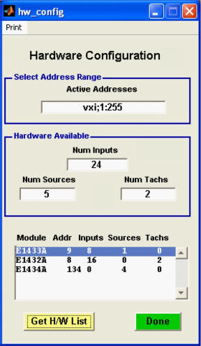 Once
the address range has been entered, click on the
Get H/W List
pushbutton to interrogate the VXI
hardware for what modules were found with that particular
address range. In this example we found an E1433A at address
9, an E1432A at an address of 8 and a E1434A at address 134 giving
us 24 input channels, 5 source channels and 2 Tachometer channels .
Once
the address range has been entered, click on the
Get H/W List
pushbutton to interrogate the VXI
hardware for what modules were found with that particular
address range. In this example we found an E1433A at address
9, an E1432A at an address of 8 and a E1434A at address 134 giving
us 24 input channels, 5 source channels and 2 Tachometer channels .
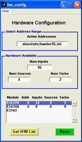
Hardware Simulate Mode: By typing "simulate;filename" in the Active address box you can setup a future test without having the measurement hardware present. This is very useful for another member of the team to be able to setup a test while the hardware is being used elsewhere. A large channel count test has a lot of operator input required to enter the parameters for each active channel (including: Point ID, Coupling, Input Mode, Transducer Model number & Serial number, Transducer Sensitivity, Engineering Units and Point Direction). Once entered, this data can be saved away in a measurement state. When hardware is available one can then load all these tedious parameters with a simple recall state.
 Clicking
the
File
pushbutton in the main
Acq_Mat
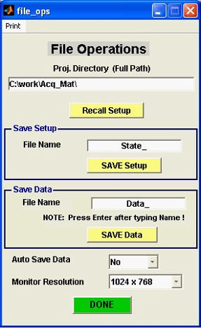
GUI brings up the window
wherein a Project Directory can be created. By doing so, all
measurement data and measurement states can be stored in a common
directory. This GUI is also where one selects the name
for any Data files or State files and actually perform the saving
function. Acq_Mat
also has a feature that allows Data to be automatically saved
at the end of each measurement. This GUI is also where
you can optimize the way
Acq_Mat utilizes the host screen
resolution by setting the Monitor Resolution to match the current
host's capability.
Clicking
the
File
pushbutton in the main
Acq_Mat
GUI brings up the window
wherein a Project Directory can be created. By doing so, all
measurement data and measurement states can be stored in a common
directory. This GUI is also where one selects the name
for any Data files or State files and actually perform the saving
function. Acq_Mat
also has a feature that allows Data to be automatically saved
at the end of each measurement. This GUI is also where
you can optimize the way
Acq_Mat utilizes the host screen
resolution by setting the Monitor Resolution to match the current
host's capability.
Checks are also made to prevent over writing existing files.
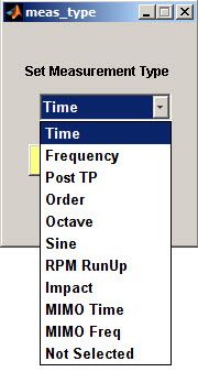 By
clicking on the
Meas Types
pushbutton in the main
Acq_Mat
GUI, one selects the measurement
type to be performed.
This approach simplifies the next step of selecting the measurement
parameters that are meaningful to the particular measurement task.
This also speeds up the setup process by minimizing operator
interaction and confusion.
Only those hardware parameters that are required for the
particular measurement type are presented to the user in the
parameter setup GUI.
By
clicking on the
Meas Types
pushbutton in the main
Acq_Mat
GUI, one selects the measurement
type to be performed.
This approach simplifies the next step of selecting the measurement
parameters that are meaningful to the particular measurement task.
This also speeds up the setup process by minimizing operator
interaction and confusion.
Only those hardware parameters that are required for the
particular measurement type are presented to the user in the
parameter setup GUI.
 Once
the measurement type is chosen, clicking on
Set Parameters
brings up the measurement
specific GUI (Time Parameters in this case) wherein the
measurement parameters needed to perform a Time Measurement are
set.
Once
the measurement type is chosen, clicking on
Set Parameters
brings up the measurement
specific GUI (Time Parameters in this case) wherein the
measurement parameters needed to perform a Time Measurement are
set.
 Within
the Time Meas Parameters
GUI, the global sampling rate
Clock Frequency
and
Span Frequency
are set.
Block Sizes
can be chosen from 64 to 8192 in
powers of 2. You can also choose the
Data Mode
to be Continuous instead of
Block. Continuous acquisition has advantages if custom
analysis is to be performed in a post test mode. The advantage
is that there are no data gaps in-between the blocks of data saved
to memory and disk, the data is contiguous.
Within
the Time Meas Parameters
GUI, the global sampling rate
Clock Frequency
and
Span Frequency
are set.
Block Sizes
can be chosen from 64 to 8192 in
powers of 2. You can also choose the
Data Mode
to be Continuous instead of
Block. Continuous acquisition has advantages if custom
analysis is to be performed in a post test mode. The advantage
is that there are no data gaps in-between the blocks of data saved
to memory and disk, the data is contiguous.
The # of Scans parameter determines the number of blocks of data that are obtained from all channels. You can choose to save all the data from all scans or just the last scan. From the File GUI invoked from the main Acq_Mat GUI (not shown here) you can also set Auto Save to Yes, allowing the data to automatically be saved with an incrementing file name strategy. That way, no time is lost in-between measurements when manually saving the data. The File GUI also allows one to save and recall measurement States and set the screen resolution of the monitor to optimize the screen real-estate.
You can elect to also save the data in SDF format in addition to the standard MATLAB® structures.
Auto Ranging allows ranging to be done in both directions (up and down allowing full scale ranges to increase or decrease) or just up ranging.
Any change to the Span, Clock Freq or Block Size will update the Sampling Summary parameters (Delta Time, Block Time, Total Scan Time & Delta Freq) in the GUI to remind you of the measurement parameters.
In the current release you can now elect to select a reduced number of Active Channels from what is physically available with a module. With multiple modules, the number of Active Channels will start from the left most module and move to the right, module wise, until the number of Active Channels is satisfied.
One can now not only display the time data while the measurement is running, but electively choose to display the Spectrums as well.
Throughput data in real time to either the Host Disk, Host RAM or the VT2216 Throughput disk. By selecting either Host Disk or ThruPut to 2216 from the Throughput to Disk pop-up you direct the data to be written to a file on the Host disk or the N2216 SCSI Throughput Disk Module. Data can be written @ > 2 MSample /Sec contiguously to the Host disk for a finite amount of time (see table on the Time Data page) or data can be written sustained @ > 5 MSamples /Sec to the internal 73 GB disk of the VT2216, without any gaps in the time record. Acq_Mat tries to simplify the User's tasks by performing some needed choices in the setup automatically. For instance, to perform throughput to the N2216, the Data Mode must be in continuous, so Acq_Mat makes this choice for you, automatically. It also notifies the user that it changed this setting and updates the GUI to reflect this.
While writing throughput data to the Host Disk, you can select via the Acq_Mat Display button how many traces are being displayed while the measurement is running.
When throughputting data to the N2216 SCSI Disks, Acq_Mat also monitors the data acquisition by sending data to the host on a time available basis. In this manner, the operator has confidence that the data being written to the N2216 is valid, good data. While in the monitoring mode, only a subset of the data being continuously written to the N2216 is available, consequently the Save All Data and Save SDF GUI choices are disabled, hence the grayed out GUI buttons.
Any ADC Overloads during the entire acquisition (all channels and all scans) are saved with the data so when post processing you know the validity of the data. If overloads do occur a unique display window will inform you of which channels are overloaded.
For maximum throughput performance to Host Disk, you can choose to turn off the data displays while the measurement is acquiring data.
Once the measurement parameters are set, clicking on Setup Inputs in the main GUI allows the input channels to be configured.
In this example, only a single VT1433 module was found within the specified address range and the Setup Input Parameters GUI shows the eight channels available to the measurement.
To change the Range of an individual channel, click on the channel number row (or use the Change Chan # entry) and then select from the pop-up window an appropriate range value. Now, if you want to globally set all the channels to this range value, click on the Range pushbutton (above the range value column).
New to the later releases is the ability to select all the channel parameters by importing an Excel file with all this data. Example Excel files are provided.
 Now,
clicking on
Setup Sources
in the
Acq_Mat
GUI allows the source channel to
be configured. Included in the source channel setup are
built-in excitation types.
Now,
clicking on
Setup Sources
in the
Acq_Mat
GUI allows the source channel to
be configured. Included in the source channel setup are
built-in excitation types.
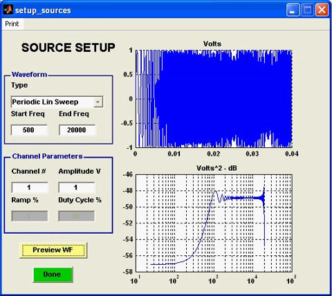
i>Acq_Mat allows the user to control the characteristics of the selected waveform (where appropriate) with start and stop frequencies and the amplitude. Acq_Mat then allows a preview of the waveform’s characteristics before it is actually used in the measurement. In the attached example, you will notice that the Ramp % and Duty Cycle % pushbuttons are ghosted out since they are not appropriate parameters when a periodic waveform is selected.
Here we see the spectral characteristics of the Log Swept Sine Wave with the starting and ending frequencies specified. The log sweep rate produces an amplitude spectrum that has similar characteristics to "pink noise" in regard to the amplitude roll-off rate.
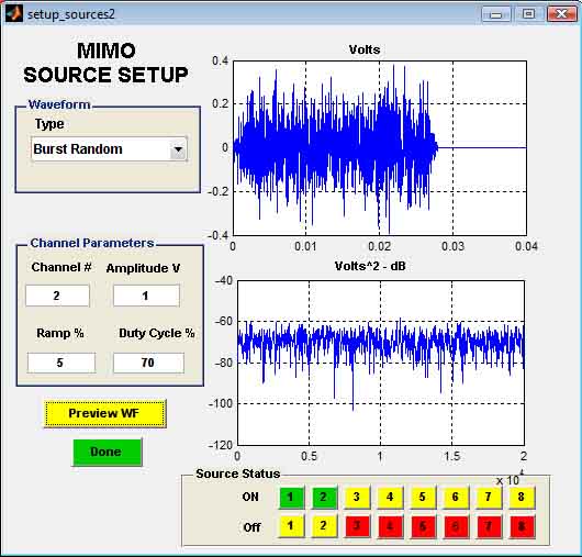
For the Multiple Input Multiple Output (MIMO) measurement the MIMO Source Setup changes to the Acq_Mat GUI shown on the left. Your choices of excitation type are Uncorrelated Burst Random and Uncorrelated Random
 To
actually start a measurement once the parameters are set, click on
Meas Control
in the main
Acq_Mat
GUI.
Then simply click on
meas_control's Start
button.
If you decide the measurement isn't
going as expected, simply click on the
Abort
button. Clicking on
Stop
will allow the data accumulated
up to this point to be saved to disk along with all setup parameters
and any overload data.
To
actually start a measurement once the parameters are set, click on
Meas Control
in the main
Acq_Mat
GUI.
Then simply click on
meas_control's Start
button.
If you decide the measurement isn't
going as expected, simply click on the
Abort
button. Clicking on
Stop
will allow the data accumulated
up to this point to be saved to disk along with all setup parameters
and any overload data.
A measurement Status box in the top of the meas_control GUI gives the current status of the hardware as the measurement proceeds.
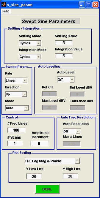 There
are a number of
Acq_Mat
GUI's not shown in this overview. Each measurement type has
its own measurement parameter setup GUI.
Here, for example, is the Swept Sine setup GUI.
During any
Acq_Mat session, any
measurement type can be performed without restarting the
Acq_Mat
program. As you switch back to a measure type you have already
made, that last setup is automatically recalled.
There
are a number of
Acq_Mat
GUI's not shown in this overview. Each measurement type has
its own measurement parameter setup GUI.
Here, for example, is the Swept Sine setup GUI.
During any
Acq_Mat session, any
measurement type can be performed without restarting the
Acq_Mat
program. As you switch back to a measure type you have already
made, that last setup is automatically recalled.
 At
left is a sample 16 trace plot which updates during the measurement.
The on-line Display
GUI allows one to chose 2, 4, 8 or 16 traces. Here we
are looking at Frequency Responses with Magnitude and Phase.
At
left is a sample 16 trace plot which updates during the measurement.
The on-line Display
GUI allows one to chose 2, 4, 8 or 16 traces. Here we
are looking at Frequency Responses with Magnitude and Phase.
The Display Setup GUI allows one to choose the number of traces to be displayed during the on-line measurement process, as well as, which display group to display. If Time measurements are being made then each trace represents one channel. Setting the number of traces to 16 and the display group to 2 will display channels 17 thru 32. Once the measurement is completed, this same GUI can be used to look through all the data with whatever number of traces. In this post measurement display mode additional display features are presented with pop-ups.
Shown here is the Setup Parameters window for the Multiple Reference Impact Option.
As you choose the Force and Response windows that will be used in subsequent measurements one can see in the time domain what the particular parameter settings look like.
If the "Save All Data" drop down list is set to "Yes" then along with the Frequency Response Functions, one can save all the impact time records if you need to prove post test that the impact data was good quality.
 After
an impact this window pops up before one accepts or rejects a
particular impact. Here we have chosen to display 4 channels
(it could have been 8 or 2 channels). Group 1 was picked so we see
the first four channels. The top four traces are the windowed
time records and the second four traces are the spectrums in Log
Magnitude format. Here one looks for an impact time record
without any double hits. A good hit will typically produce a
spectrum as shown in the third trace from the top on the left hand
side. Accepting this record will add it to average, based upon
the number of averages specified.
After
an impact this window pops up before one accepts or rejects a
particular impact. Here we have chosen to display 4 channels
(it could have been 8 or 2 channels). Group 1 was picked so we see
the first four channels. The top four traces are the windowed
time records and the second four traces are the spectrums in Log
Magnitude format. Here one looks for an impact time record
without any double hits. A good hit will typically produce a
spectrum as shown in the third trace from the top on the left hand
side. Accepting this record will add it to average, based upon
the number of averages specified.
 At
left is the next plot shown after
"Accepting" an impact for what
happens to be a different Input Point number.
At
left is the next plot shown after
"Accepting" an impact for what
happens to be a different Input Point number.
After an Impact is "Accepted" the window changes to the Averaged Frequency Response Functions with Log Magnitude and Phase plots. The channel annotations are done automatically by using the setup parameters (Channel #, point and direction).
 To
change the input point number for the next measurement, simply click
on "Incr Point #" in the meas_control
window. Incrementing this point number will follow the
sequence that was imported from the Excel Spreadsheet during the
Setup Inputs phase.
To
change the input point number for the next measurement, simply click
on "Incr Point #" in the meas_control
window. Incrementing this point number will follow the
sequence that was imported from the Excel Spreadsheet during the
Setup Inputs phase.
 One
can recall any saved data by pressing the
Saved Plot
button in the main
Acq_Mat
GUI. The GUI at left appears which
allows one to look in any project directory and by clicking on the
Recall Data button, a pop-up list of the data file names in that
project directory will appear. Double clicking on any file
name fills in the Data
Stats box. Clicking the
Multi Plot
button brings up the
Multiple Trace Plot GUI whereby
one chooses the number of traces and the data group along with the
plotting formats available. The formats available will be
dependent upon the data recalled.
One
can recall any saved data by pressing the
Saved Plot
button in the main
Acq_Mat
GUI. The GUI at left appears which
allows one to look in any project directory and by clicking on the
Recall Data button, a pop-up list of the data file names in that
project directory will appear. Double clicking on any file
name fills in the Data
Stats box. Clicking the
Multi Plot
button brings up the
Multiple Trace Plot GUI whereby
one chooses the number of traces and the data group along with the
plotting formats available. The formats available will be
dependent upon the data recalled.
 Here
the number of traces has been reduced to 4 and
Display Group 2
(channels 3 & 4) was chosen. Since the data is a Frequency
Response measurement, the first two traces show the LogMagnitude and
second two traces show the Coherence functions for an Impact
measurement.
Here
the number of traces has been reduced to 4 and
Display Group 2
(channels 3 & 4) was chosen. Since the data is a Frequency
Response measurement, the first two traces show the LogMagnitude and
second two traces show the Coherence functions for an Impact
measurement.
Dual cursors are automatically displayed after a measurement is completed
 Here
a post test plot of one of the saved Impact Responses from the data
base accumulated during an Multi-Reference Impact test. One
can electively save along with all the frequency responses the time
records of all the individual impact records for all channels and
all impact averages. Both the raw time records and the force
and response windowed times records are saved.
Here
a post test plot of one of the saved Impact Responses from the data
base accumulated during an Multi-Reference Impact test. One
can electively save along with all the frequency responses the time
records of all the individual impact records for all channels and
all impact averages. Both the raw time records and the force
and response windowed times records are saved.
 This
plot is an example of the Single Plot Post Test plotting capability
built into the
Saved Plot
button GUI. Here a Impact
Frequency Response Function measurement is displayed where the
operator's chosen format is a 3-D plot (real vs. imaginary vs.
frequency). The MATLAB®
toolbars allow this plot to be dynamically rotated.
This
plot is an example of the Single Plot Post Test plotting capability
built into the
Saved Plot
button GUI. Here a Impact
Frequency Response Function measurement is displayed where the
operator's chosen format is a 3-D plot (real vs. imaginary vs.
frequency). The MATLAB®
toolbars allow this plot to be dynamically rotated.
The operator can choose a number of different formats, Magnitude & Phase, Magnitude and Coherence, Log Magnitude, Real & Imaginary etc.
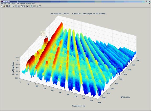 The
RPM Run-Up
Measurement at the left presents the results from a run-up on
a device with both oil-whirl and oil-whip.
The
RPM Run-Up
Measurement at the left presents the results from a run-up on
a device with both oil-whirl and oil-whip.
This measurement Requires the Acq_Mat RPM Run Up Option and the hardware tachometer Option AYF.
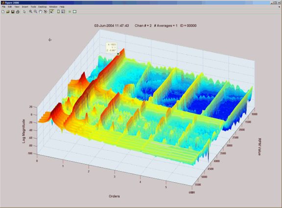 A
Computed Order Track
Measurement using the same "Device Under Test" as above is shown
here. Computed
Order Tracking allows a much easier visual interpretation of the
devices "Once per Rev" vibration response and the harmonics (Orders)
of the once per rev component.
A
Computed Order Track
Measurement using the same "Device Under Test" as above is shown
here. Computed
Order Tracking allows a much easier visual interpretation of the
devices "Once per Rev" vibration response and the harmonics (Orders)
of the once per rev component.
This measurement Requires the Acq_Mat Order Track Option and the hardware tachometer Option AYF.
If you have specific questions, send your inquiry to info@dynamic-measurements.com